Royal Belgian Institute for Aeronomy¶

Ex. #6. visualisation of a drift shell¶

Description¶

Magnetic drift shells can be built with the help of the subroutines ud310() or ud317(). To visualize the drift shells, the subroutine ut992() can be used to print the drift shell data into a file. A graphical tool can then be used to display the shell.

In the example below, we took advantage that the library can be directly linked to IDL (see FAQ G.06, and FAQ T.05). The IDL routines listed in the next section make use of the subroutine ut985() to read the magnetic drift shell stored in the common blocks uc110, uc120 and uc130. In the source code of both subroutines, it is assumed that the library has been correctly initialized, the different structures have been fully declared, and the drift shell has been successfully built by the subroutine ud310() or the subroutine ud317(). Note that the IDL routine unilib_init can be used to declare the useful structures.

The source code listed below include two IDL routines: spl_fieldline and shade_shell. The routine spl_fieldline uses natural splines to tabulate a magnetic field line segment with a given number of points. The routine shade_shell makes successive calls to the subroutine ut985() and the routine spl_fieldline in order to return a set of vertices and polygons which describe the magnetic drift shell. These vertices and polygons can be then directly use with the IDL function POLYSHADE to produce a shaded-surface representation of one or more magnetic drift shells.

Source¶

PRO spl_fieldline, field_line, tabulated_line, $
                   number=number, bmax=bmax, shade=shade
;
;   Purpose:  Tabulate a magnetic field line segment with equidistant points.
;   Arguments:
;             field_line     = an array of zseg structures
;             tabulated_line = a (3,n) array containing the X, Y, and Z
;                              coordinates of each point
;   Keywords:
;             number         = number of equidistant points (default, 20)
;             bmax           = value of the magnetic field intensity at
;                              the mirror points
;             shade          = an array, with the same number of elements
;                              as tabulated_line, that will contained the
;                              magnetic field intensity at each point
;
     IF NOT KEYWORD_SET( number ) THEN number = 20
     n      = N_ELEMENTS( field_line )
;
;    Convert to cartesian coordinates
;
     xyz    = CV_COORD( /degrees, /to_rect,                                  $
               from_sphere = TRANSPOSE( [[  field_line.beg.coord.elong ],    $
                                        [ 90-field_line.beg.coord.colat ],   $
                                        [  field_line.beg.coord.radius  ]] ) )
;
     b      = field_line.beg.b.dnrm
     arcl   = field_line.arcl
;
;
     IF KEYWORD_SET(bmax) THEN BEGIN
;
;      Constraint fieldline between mirror points
;
       k    = WHERE( fieldline.beg.b.dnrm LE bmax )
       IF k(0) LT 0 THEN k=[0]
       xyz  = xyz(*,k)
       arcl = arcl(k)
       b    = b(k)
       n    = N_ELEMENTS( k )
;
     ENDIF
;
;
     IF n LE 1 THEN BEGIN
;
       tabulated_line = xyz(*,0) # ( 1 + FLTARR( number ) )
       shade          = FLTARR( number ) + b(0)
;
     ENDIF ELSE BEGIN
;
;      Use natural splines to tabulate the field line segment
;
       arcl = arcl(n-1) + arcl(0) - arcl
;
       s    = arcl(0) + FINDGEN( number ) / ( number-1 ) * ( arcl(n-1)-arcl(0) )
       x    = SPL_INTERP( arcl, xyz(0,*), SPL_INIT( arcl, xyz(0,*) ), s )
       y    = SPL_INTERP( arcl, xyz(1,*), SPL_INIT( arcl, xyz(1,*) ), s )
       z    = SPL_INTERP( arcl, xyz(2,*), SPL_INIT( arcl, xyz(2,*) ), s )
;
       tabulated_line = TRANSPOSE( [ [x], [y], [z] ])
       shade          = SPL_INTERP( arcl, b, SPL_INIT( arcl, b ), s )
;
     ENDELSE
;
;
END

PRO poly_shell, vertices, polygons, $
                number=number, bmax=bmax, shade=shade
;
;   Purpose:  Transfer a magnetic drift shell from UNILIB to IDL in the form of
;             a shaded surface
;   Arguments:
;             vertices       = a (3,n) array containing the X, Y, and Z
;                              coordinates of each vertex of the drift shell
;             polygons       = a longword array containing the indices
;                              of the vertices for each polygon. The vertex
;                              description of each polygon is a vector of
;                              the form: [3,i0,i1,i2].
;   Keywords:
;             number         = keyword passed to spl_fieldline
;             bmax           = value of the magnetic field intensity at
;                              the mirror points
;             shade          = an array that will contained the magnetic
;                              field intensity on the drift shell
;
     IF NOT KEYWORD_SET(bmax) THEN bmax=0
     IF NOT KEYWORD_SET(number) THEN number=20
;
;    Init. a list of polygon vertices
;
     k          = INDGEN( 2 * number - 2 )
     polygon    = TRANSPOSE( [ [             3 + 0*k                ],  $
                               [          number + (k+1)/2          ],  $
                               [                k/2                 ],  $
                               [ 1 + k/2 + number * ( 1 - k mod 2 ) ] ] )
;
;    Retrieve the first field line segment
;
     length     = 100L
     mdata      = REPLICATE( {zseg}, length )
;
     kindex     = -1L
     klength    = length
     status     = CALL_EXTERNAL( 'unilib', 'UT985', kindex, klength, mdata)
     IF klength LE -999999990L THEN MESSAGE, 'call to UT985 failed'
;
     IF klength LE 0 THEN BEGIN
;
;      Adjust the size of mdata
;
       length   = 10L - klength
       mdata    = REPLICATE( {zseg}, length )
       status   = CALL_EXTERNAL( 'unilib', 'UT985', kindex, klength, mdata)
       IF klength LT 0L THEN MESSAGE, 'call to UT985 failed'
;
     ENDIF
;
;
     kend       = kindex
     spl_fieldline, mdata( 0: klength-1 ), vertices, $
                    number=number, bmax=bmax, shade=shade
     polygons   = -1L
;
;    Loop on the next field lines
;
     REPEAT BEGIN
;
;      Load a magnetic field line segment
;
       klength  = length
       status   = CALL_EXTERNAL( 'unilib', 'UT985', kindex, klength, mdata)
       IF klength LE -999999990L THEN MESSAGE, 'call to UT985 failed'
;
       IF klength LE 0 THEN BEGIN
         length = 10L - klength
         mdata  = REPLICATE( {zseg}, length )
         status = CALL_EXTERNAL( 'unilib', 'UT985', kindex, klength, mdata)
         IF klength LT 0L THEN MESSAGE, 'call to UT985 failed'
       ENDIF
;
     spl_fieldline, mdata( 0: klength-1 ), thisline, $
                    number=number, bmax=bmax, shade=thisshade
;
     IF kindex NE kend THEN BEGIN
;
;      Append the field line segment and vertex polygons
;
       vertices = [ [vertices], [thisline] ]
       shade    = [ [shade], [thisshade] ]
;
       IF polygons(0) LT 0 THEN polygons = polygon $
                           ELSE polygons = [ [polygons], [polygon] ]
;
;      Adapt polygon for the next segment
;
       polygon(1: 3, *) = polygon(1: 3, *) + number
;
     ENDIF ELSE BEGIN
;
;      Back to the first field line segment
;
       k                = WHERE( polygon ge polygon(1,0) )
       polygon(k)       = polygon(k) - polygon(1,0)
       polygons         = [ [polygons], [polygon] ]
;
     ENDELSE
;
;
  ENDREP UNTIL kindex EQ kend
;
END

Results¶

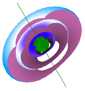
The above IDL subroutines have been used to produce the following picture where three magnetic drift shells are represented. For the sake of clarity, the shells have been cut by a plane.

../_images/try06.png — Projection of three magnetic drift shells cut by a plane.¶

Courtesy of B. Quaghebeur (BIRA) The drift shells are characterized by a shell parameter set to 2, 4 and 6, respectively, and a value of \(B_m/B_0\) fixed to 7. The cut view is realized by the plane x + y = 6,500 km (in GEO coordinates).

UNILIB/tags/v3.02